1. Multi-class Weather Dataset
https://www.kaggle.com/datasets/pratik2901/multiclass-weather-dataset
Multi-class Weather Dataset은 다양한 기상 조건을 포함하는 이미지 데이터셋으로, 주로 기계 학습 및 딥러닝 모델을 학습하거나 평가하는 데 사용됩니다. 이 데이터셋은 맑음, 비, 눈, 흐림과 같은 여러 날씨 유형으로 라벨이 지정된 다중 클래스 분류 문제를 다룹니다. 각 클래스는 다양한 시간대, 계절, 지역에서 촬영된 이미지를 포함하여 현실 세계의 다양성을 반영하도록 설계되었습니다. 이를 통해 모델은 날씨 조건을 정확히 분류하고, 기상 관측, 자동화된 날씨 보고, 혹은 자율주행 차량의 환경 인식 시스템과 같은 다양한 응용 분야에서 활용될 수 있습니다.
Multi-class Weather Dataset
Image Dataset provides a platform for recognizing different weather conditions.
www.kaggle.com
!kaggle datasets download pratik2901/multiclass-weather-dataset
Dataset URL: https://www.kaggle.com/datasets/pratik2901/multiclass-weather-dataset
License(s): Attribution 4.0 International (CC BY 4.0)
Downloading multiclass-weather-dataset.zip to /content
 92% 84.0M/91.4M [00:00<00:00, 158MB/s]
100% 91.4M/91.4M [00:00<00:00, 142MB/s]
import os
import zipfile
import random
from shutil import copyfile,rmtree
zip_file = 'multiclass-weather-dataset.zip'
base_dir = './Multi-class Weather Dataset'
train_dir = './train'
test_dir = './test'
extract_path = '.' #그자리에 폴더없이 압축 폴더 풀게하려고 만든 경로
with zipfile.ZipFile(zip_file, 'r') as zip_ref:
    zip_ref.extractall(extract_path) #압축 전체 풀기
# 분류 디렉토리 목록
categories = ['Cloudy','Rain','Shine','Sunrise']
if os.path.exists(train_dir):
    rmtree(train_dir)
if os.path.exists(test_dir):
    rmtree(test_dir)
os.makedirs(train_dir, exist_ok=True)
os.makedirs(test_dir, exist_ok=True)
for category in categories:
    os.makedirs(os.path.join(train_dir, category), exist_ok=True)
    os.makedirs(os.path.join(test_dir, category), exist_ok=True)
from posixpath import split
#각 카테고리별 데이터 파일 나누기
for category in categories:
    category_path = os.path.join(base_dir, category) #파일있는 디렉토리 위치 지정
    files = os.listdir(category_path) #디렉토리 안에 들어있는 파일 폴더 리스트 형식으로 가져옴

    #데이터 섞기
    random.shuffle(files)

    #데이터 8:2로 나누기
    split_idx = int(len(files) * 0.8)
    train_files = files[:split_idx]
    test_files = files[split_idx:]

    #파일 복사
    for file in train_files:
        src = os.path.join(category_path, file)
        dst = os.path.join(train_dir, category, file) # 폴더명,카테고리명,파일명 합치기
        copyfile(src, dst)

    for file in test_files:
        src = os.path.join(category_path, file)
        dst = os.path.join(test_dir, category, file) # 폴더명,카테고리명,파일명 합치기
        copyfile(src, dst)

print('데이터 분리 완료!')
import torch
import time
import torchvision
import torchvision.transforms as transforms
import torchvision.models as models
import torchvision.datasets as datasets
from torchvision.utils import make_grid

import torch.optim as optim
import torch.nn as nn
import torch.nn.functional as F # 딥러닝 관련 함수 모아둔것
from torch.utils.data import random_split
from torch.utils.data import DataLoader


import matplotlib.pyplot as plt
import matplotlib.image as mpimg
import numpy as np
#객체 만들기
#Compose 변환이 있다면 차례대로 적용 데이터 증강 argu 처럼 랜덤으로 적용이 있고 아닌게 있음
transform_train = transforms.Compose([
    transforms.Resize((256, 256)), #무조건 적용하는거 랜덤 적용 아님 이미지나 영상 사이즈 바꾸기
    transforms.RandomHorizontalFlip(), #랜덤으로 좌우 반전 확률 50%
    transforms.ToTensor(),#무조건 적용
    transforms.Normalize(
        mean=[0.5, 0.5, 0.5],
        std=[0.5, 0.5, 0.5]
    )# 0~1인 양수값으로만 정규화가 아닌 -1 ~ 1사이 값으로 정규화 하기 위해서 사용. 렐루를 위해서 정규화 하는게 편함 렐루는 0이하의 값을 날리는데 그걸 통해서 학습속도를 높히려고 하는것

])

transform_test = transforms.Compose([
    transforms.Resize((256, 256)), #무조건 적용하는거 랜덤 적용 아님 이미지나 영상 사이즈 바꾸기
    # transforms.RandomHorizontalFlip(), # 테스트는 변경할 필요 없기 때문에 삭제
    transforms.ToTensor(),#무조건 적용
    transforms.Normalize(
        mean=[0.5, 0.5, 0.5],
        std=[0.5, 0.5, 0.5]
    )# 0~1인 양수값으로만 정규화가 아닌 -1 ~ 1사이 값으로 정규화 하기 위해서 사용. 렐루를 위해서 정규화 하는게 편함 렐루는 0이하의 값을 날리는데 그걸 통해서 학습속도를 높히려고 하는것

])
transforms.ToTensor()
- 이미지를 PyTorch 텐서(tensor)로 변환합니다.
- 이미지의 픽셀 값을 [0, 255] 범위에서 [0.0, 1.0] 범위로 정규화합니다.
- 이미지의 차원을 (H, W, C) 형식에서 PyTorch에서 사용하는 (C, H, W) 형식으로 바꿉니다.
- H: 이미지의 높이 (Height)
- W: 이미지의 너비 (Width)
- C: 채널(Channel; 예: RGB 이미지의 경우 3,흑백은 1)
transforms.Normalize(mean, std)
- 텐서로 변환된 이미지의 픽셀 값을 정규화(normalization)합니다.
- mean: 각 채널(R, G, B)의 평균값.
- std: 각 채널의 표준편차.
- mean=[0.5, 0.5, 0.5]: R, G, B 채널 각각의 평균을 0.5로 설정.(평균을 억지로 0.5로 해서 -1~1로 변환하는거)
- std=[0.5, 0.5, 0.5]: R, G, B 채널 각각의 표준편차를 0.5로 설정.
- 이 정규화는 일반적으로 픽셀 값의 범위를 [−1,1][-1, 1][−1,1]로 조정하기 위해 사용됩니다. (픽셀 값이 [0,1][0, 1][0,1]로 변환된 상태에서)
train_dataset = datasets.ImageFolder(
    root='train/',
    transform=transform_train
)

dataset_size = len(train_dataset)
train_size = int(dataset_size * 0.8) # valid데이터 검증데이터로 뽑기 위해서 다시 80% 뽑아서 train_size만들기
val_size = dataset_size - train_size #전체에서 80%빼서 검증 데이터 val_size만들기
ImageFolder
- datasets.ImageFolder는 이미지 데이터를 특정 디렉터리 구조에서 로드하는 클래스입니다.
- 디렉터리 이름을 레이블(class label)로 간주하며, 각 디렉터리 내의 이미지 파일들을 해당 레이블에 할당합니다. # 폴더이름이 분류할때의 클래스 이름이 됨
- 이 클래스는 이미지 데이터를 PyTorch 데이터셋(Dataset) 형식으로 변환하므로, DataLoader와 함께 사용하여 배치 처리 및 데이터 증강(data augmentation)을 쉽게 적용할 수 있습니다.
train_dataset, val_dataset = random_split(train_dataset, [train_size, val_size]) # train_dataset을 둘로 랜덤하게 나눠서 train_dataset, val_dataset여기에 넣기
test_dataset = datasets.ImageFolder(
    root='test/',
    transform=transform_test
)
#테스트 데이터는 나눌필요없으니까 지정만
train_dataloader = DataLoader(train_dataset, batch_size=64, shuffle=True)# 학습 데이터
val_dataloader = DataLoader(val_dataset, batch_size=64, shuffle=True) # 검증 데이터
test_dataloader = DataLoader(test_dataset, batch_size=64, shuffle=False) # 테스트 데이터는 섞을 필요없으니까 False
plt.rcParams['figure.figsize'] = [12, 8] #크기 rcParams로고정
plt.rcParams['figure.dpi'] = 60 # dpi해상도
plt.rcParams.update({'font.size': 20})
def imshow(input):
    # torch.Tensor => numpy
    input = input.numpy().transpose((1, 2, 0)) #numpy로 데이터 ndarr로 변환 ,transpose()차원 순서 바꾸기 C W H순서를 바꾸기 위해서 사용 input에 재저장 HWC ->CHW
    mean = np.array([0.5, 0.5, 0.5])
    std = np.array([0.5, 0.5, 0.5])
    input = std * input + mean # 정규화 해제 (역정규화) 원래대로 돌림
    input = np.clip(input, 0, 1) #np.clip(input, 0, 1) 값이 0보다 작은 경우 0, 1보다 큰 경우 1로 변환합니다.
    plt.imshow(input) # 0~1로 찍어도 원래대로 0~255로 다시 찍어주는 기능이 있기때문에 -1~1로 정규화 한 값을 0~1로 역 정규화 한것
    plt.show()
class_names = {
    0: 'Cloudy',
    1: 'Rain',
    2: 'Shine',
    3: 'Sunrise'
}
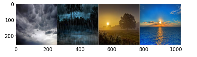
iterator = iter(train_dataloader) #데이터를 반복시킬수 있는 순차 객체로 만들어줌
imgs, labels = next(iterator) # 하나만 집어옴
out = make_grid(imgs[:4]) # 여러 이미지를 하나의 격자(grid) 형태로 합칩니다. 출력 이미지의 기본 배치는 가로로 나열된 이미지이며, 간격은 기본적으로 2 픽셀입니다.
imshow(out)
print([class_names[labels[i].item()] for i in range(4)])
['Cloudy', 'Rain', 'Sunrise', 'Sunrise']
2. 다양한 모델 만들기
# 단일 선형 계층
# 활성화 함수나 추가 계층이 없으므로 모델이 표현할 수 있는 함수는 단순 선형 변환에 제한
# 전체 파라미터 수 : (256*256*3+1)*4 = 786,436
# 입력:256*256*3 ,바이오스:1 ,나가는쪽 웨이트:*4
# 파라미터 개수가 많으면 성능이 좋다 대신 오래걸림 파라미터가 표현력이라 보면 됨
# 비선형적 특징이 있어서 학습을 잘 못할 가능성이 있음 (표현이 복잡한 데이터를 학습하기 어려움)

class Model1(nn.Module): # nn.Module 상속받아서 쓰기
    def __init__(self):
        # super 부모클래스에 내 클래스 이름 넘겨서 생성자 호출
        super(Model1, self).__init__()
        self.linear1 = nn.Linear(256*256*3,4) #256*256*3: 컬러사진,4 : 클래스는 4개(날씨)
        self.flatten = nn.Flatten()

    def forward(self, x):
        x = self.flatten(x) #x에 이미지 넣은거 일렬로 만들어 주기 (이미지가 좌표가 중요한데 1차원이 되면서 좌표가 사라지니까 일반적인 딥러닝으로는 결과가 별로 좋지 않음)
        x = self.linear1(x)
        return x
# 두 개의 선형 계층을 사용하여 입력 데이터를 단계적으로 압축
# 활성화 함수가 없으므로 각 계층간 변환은 선형적
# 전체 파라미터 수 : (256*256*3+1)*64 + (64 + 1)*4 = 12,583,236

class Model2(nn.Module):
    def __init__(self):
        super(Model2, self).__init__()
        self.linear1 = nn.Linear(256*256*3,64) # 파라미터가 늘었으니 웨이트가 늘어서 더 많은 계산을 하게 됨
        self.linear2 = nn.Linear(64,4)
        self.flatten = nn.Flatten()

    def forward(self, x):
        x = self.flatten(x)
        x = self.linear1(x)# 이미지 64개로 내보냄
        x = self.linear2(x)# 64개로 내보냈으니 64로 받고 4로 내보냄
        return x
# 다중구조와 ReLu활성화 함수를 사용하여 비선형적 특징을 학습할 수 있음
# Dropout을 통해서 과적합 방지
# (256*256*3+1)*128 + (128 + 1)*64 + (64+1)*32 + (32+1)*4 = 25176420

class Model3(nn.Module):
    def __init__(self):
        super(Model3, self).__init__()
        self.linear1 = nn.Linear(256*256*3,128) #128로 압축해서 내보냄
        self.dropout1 = nn.Dropout(0.5) # 다음으로 넘어가는 파라미터를 써준 확률(0.5 (50%))로 꺼줌 한 가중치만 트레이닝에 국한되지 않도록 해서 나머지 가중치로 갱신 (과적합 방지)
        self.linear2 = nn.Linear(128, 64)
        self.dropout2 = nn.Dropout(0.5)
        self.linear3 = nn.Linear(64, 32)
        self.dropout3 = nn.Dropout(0.5)
        self.linear4 = nn.Linear(32, 4)
        self.flatten = nn.Flatten()

    def forward(self, x):
        x = self.flatten(x) # 일단 입력데이터 1차원으로 변환

        x = F.relu(self.linear1(x)) #196608차원의 입력을 128차원으로 축소 -> ReLu활성화
        # 하나의 레이어가 끝날때 마다 하나의 레이어를 추가하게해서 비선형으로 만들어줌
        #리니어1을 통과한 다음에 렐루로 감싸서 보냄
        x = self.dropout1(x)# 과적합 방지를 위해 0.5확률로 무작위로 비활성화

        x = F.relu(self.linear2(x))#128차원의 입력을 64차원으로 축소 -> ReLu활성화
        # 두번째 레이어 두번째 리니어로 또 리니어2> 렐루에 통과 > 보내기
        x = self.dropout2(x)# 과적합 방지를 위해 0.5확률로 무작위로 비활성화

        x = F.relu(self.linear3(x))#64차원의 입력을 32차원으로 축소 -> ReLu활성화
        x = self.dropout3(x)# 과적합 방지를 위해 0.5확률로 무작위로 비활성화
        x = self.linear4(x)# 최종출력
        # 마지막 리니어4통과 해서 결과 만들기
        # 활성화 함수를 종류를 섞어 쓰지 않는 이유는 뒤로 미분할때 탄젠트나 시그모이드는 기울기 소실때문에 안쓰는거라 굳이 안섞어 쓰는것임
        return x
nn.Module 상속
모델 구성 요소 관리: 레이어와 파라미터를 자동으로 관리. 순전파(Forward) 정의: forward() 메서드를 통해 간단하고 일관된 순전파 과정 정의. 계층적 설계: 서브모듈을 활용해 복잡한 모델을 쉽게 설계. 유틸리티 제공: 파라미터 저장/로드, 학습/추론 모드 전환 등 다양한 기능 제공. PyTorch 호환성: 최적화, 데이터 로더 등 PyTorch의 다른 기능과 손쉽게 통합. 추상화: 저수준 작업을 추상화하여 개발자의 생산성을 향상.
Dropout
nn.Dropout()은 PyTorch에서 제공하는 과적합(overfitting)을 방지하기 위한 레이어입니다. 드롭아웃은 학습 과정 중 일부 뉴런을 무작위로 "비활성화(drop)"함으로써, 모델이 특정 뉴런에 지나치게 의존하지 않도록 도와줍니다. 이를 통해 모델의 일반화 성능이 향상됩니다.
(256*256*3+1)*128 + (128 + 1)*64 + (64+1)*32 + (32+1)*4
25176420256*256*3
196608# 에포크 돌릴때 한번씩 실행 시키려는 함수
def train():
start_time = time.time()
print(f'[Epoch: {epoch + 1} - Training]')
model.train() #모델을 학습모드로 전환 그래데이션,.? 아무튼 벨리데이션이나 테스트 모드로 할때 오류 안나게
# 학습, 드롭아웃, 배치, 정규화등 학습 시에만 활성화하도록
#초기화
total = 0 #학습 데이터 수
running_loss = 0.0 #배치단위 로스값 손실값
running_corrects = 0 #배치단위 맞춘 예측 개수 라벨하고 정답을 얼마나 맞췄는지
for i, batch in enumerate(train_dataloader):
imgs, labels = batch #(imgs, labels)
imgs, labels = imgs.cuda(), labels.cuda() #GPU로 계산하도록
outputs = model(imgs) # 모델에 넣어서 계산
optimizer.zero_grad() # 기울기 초기화
_, preds = torch.max(outputs, 1) # 열중에 가장 높은 값을 뽑아서 preds 근데 로짓값이 나옴
loss = criterion(outputs, labels) #로스값 계산 크로스엔트로피 로스값 즉 라벨이랑 로짓값이 얼마나 차이나는지 저장
loss.backward() # 역전파
optimizer.step() # W, B 기울기 갱신
total += labels.shape[0] # 라벨을 하나씩 가져오기때문에 몇개의 데이터를 처리중인지 누적해서 셀수 있음
running_loss += loss.item()
running_corrects += torch.sum(preds == labels.data) #예측값과 라벨 데이터값과 일치한지 계산
if (i==0) or (i % log_step == log_step - 1):
print(f'[Batch: {i + 1}] running train loss: {running_loss / total}, running train accuracy: {running_corrects / total}')
#에폭 프린트 처리
print(f'test loss:{running_loss / total}, accuracy: {running_corrects / total}')
print("elapsed time:", time.time() - start_time)
return running_loss / total, (running_corrects / total).item()
def adjust_learning_rate(optimizer, epoch):
    lr = learning_rate
    if epoch >= 3: #3보다 커지면 10으로 나눠서 learning_rate 조절
        lr /= 10
    if epoch >= 7:
        lr /= 10
    # optimizer.param_groups : 옵티마이저는 학습률과 관련된 파라미터 그룹을 관리
    # lr키로 학습률 값이 설정
    for param_group in optimizer.param_groups:
        param_group['lr'] = lr # 미리 설정되어있는 학습률을 대신해 내가 설정한 lr값을 계속 넣어줌 lr값을 내가 설정한걸로 바꿔주는것
def validate():
    start_time = time.time()
    print(f'[Epoch: {epoch + 1} - Validation]')
    model.eval() #모델을 검증모드로 변경

    #초기화
    total = 0               #학습 데이터 수
    running_loss = 0.0      #배치단위 로스값 손실값
    running_corrects = 0    #배치단위 맞춘 예측 개수 라벨하고 정답을 얼마나 맞췄는지

    for i, batch in enumerate(val_dataloader):
        imgs, labels = batch                        #(imgs, labels)
        imgs, labels = imgs.cuda(), labels.cuda()   #GPU로 계산하도록


        with torch.no_grad():
            outputs = model(imgs) # 모델에 넣어서 계산
            _, preds = torch.max(outputs, 1) # 열중에 가장 높은 값을 뽑아서 preds 근데 로짓값이 나옴
            loss = criterion(outputs, labels) #로스값 계산 크로스엔트로피 로스값 즉 라벨이랑 로짓값이 얼마나 차이나는지 저장

            total += labels.shape[0] # 라벨을 하나씩 가져오기때문에 몇개의 데이터를 처리중인지 누적해서 셀수 있음
            running_loss += loss.item()
            running_corrects += torch.sum(preds == labels.data) #예측값과 라벨 데이터값과 일치한지 계산

            if (i==0) or (i % log_step == log_step - 1):
                print(f'[Batch: {i + 1}] running val loss: {running_loss / total}, running val accuracy: {running_corrects / total}')

    #에폭 프린트 처리
    print(f'val loss:{running_loss / total}, accuracy: {running_corrects / total}')
    print("elapsed time:", time.time() - start_time)

    return running_loss / total, (running_corrects / total).item()
def test():
    start_time = time.time()
    print(f'[Test]')
    model.eval() #모델을 검증모드로 변경

    #초기화
    total = 0               #학습 데이터 수
    running_loss = 0.0      #배치단위 로스값 손실값
    running_corrects = 0    #배치단위 맞춘 예측 개수 라벨하고 정답을 얼마나 맞췄는지

    for i, batch in enumerate(test_dataloader):
        imgs, labels = batch                        #(imgs, labels)
        imgs, labels = imgs.cuda(), labels.cuda()   #GPU로 계산하도록


        with torch.no_grad():
            outputs = model(imgs) # 모델에 넣어서 계산
            _, preds = torch.max(outputs, 1) # 열중에 가장 높은 값을 뽑아서 preds 근데 로짓값이 나옴
            loss = criterion(outputs, labels) #로스값 계산 크로스엔트로피 로스값 즉 라벨이랑 로짓값이 얼마나 차이나는지 저장

            total += labels.shape[0] # 라벨을 하나씩 가져오기때문에 몇개의 데이터를 처리중인지 누적해서 셀수 있음
            running_loss += loss.item()
            running_corrects += torch.sum(preds == labels.data) #예측값과 라벨 데이터값과 일치한지 계산

            if (i==0) or (i % log_step == log_step - 1):
                print(f'[Batch: {i + 1}] running test loss: {running_loss / total}, running test accuracy: {running_corrects / total}')

    #에폭 프린트 처리
    print(f'test loss:{running_loss / total}, accuracy: {running_corrects / total}')
    print("elapsed time:", time.time() - start_time)

    return running_loss / total, (running_corrects / total).item()
# 초기화
learning_rate = 0.01
log_step = 11
model = Model1()
model = model.cuda()
criterion = nn.CrossEntropyLoss()
optimizer = optim.SGD(model.parameters(), lr=learning_rate, momentum=0.9) # momentum : 아담에서 설정되어있는 값 처음에는 많이씩 움직이다가 값을 조절해서 점점 조금씩 가게하는 그거
# 처음에 준 러닝 래이트 값을 확인해서 그다음에는 그 값의 90퍼센트로 하게 함 0,1,2,바퀴는 그대로 돌고 점점 내가 설정한 값으로 바뀜
num_epochs = 20
best_val_acc = 0
best_epoch = 0

history = []
accuracy = []
# Ensure weights directory exists
os.makedirs("weights", exist_ok=True)

for epoch in range(num_epochs):
    adjust_learning_rate(optimizer, epoch)
    train_loss, train_acc = train()
    val_loss, val_acc = validate()
    history.append((train_loss, val_loss))
    accuracy.append((train_acc, val_acc))
    if val_acc > best_val_acc:
        print('[info] best validation accuracy!')
        best_val_acc = val_acc
        best_epoch = epoch
        torch.save(model.state_dict(), f'weights/best_checkpoint_epoch_{epoch + 1}.pth')

torch.save(model.state_dict(),f'weights/last_checkpoint_epoch_{epoch + 1}.pth')
[Epoch: 1 - Training]
[Batch: 1] running train loss: 0.2811339497566223, running train accuracy: 0.6875
[Batch: 11] running train loss: 0.2387916405092586, running train accuracy: 0.7002841234207153
test loss:0.25128902414080495, accuracy: 0.7023643851280212
elapsed time: 5.401939153671265
[Epoch: 1 - Validation]
[Batch: 1] running val loss: 0.25604507327079773, running val accuracy: 0.71875
val loss:0.2728432602352566, accuracy: 0.7666667103767395
elapsed time: 1.270921230316162
[info] best validation accuracy!
[Epoch: 2 - Training]
[Batch: 1] running train loss: 0.1276315599679947, running train accuracy: 0.859375
[Batch: 11] running train loss: 0.23266666314818643, running train accuracy: 0.7684659361839294
test loss:0.31176773994456414, accuracy: 0.7663421630859375
elapsed time: 6.2567243576049805
[Epoch: 2 - Validation]
[Batch: 1] running val loss: 0.2564195990562439, running val accuracy: 0.8125
val loss:0.40562044779459633, accuracy: 0.7388889193534851
elapsed time: 1.2428276538848877
[Epoch: 3 - Training]
[Batch: 1] running train loss: 0.32056573033332825, running train accuracy: 0.734375
[Batch: 11] running train loss: 0.28933957760984247, running train accuracy: 0.7357954978942871
test loss:0.3047118591499594, accuracy: 0.7357441186904907
elapsed time: 5.408267021179199
[Epoch: 3 - Validation]
[Batch: 1] running val loss: 0.402869313955307, running val accuracy: 0.65625
val loss:0.42946723302205403, accuracy: 0.6888889074325562
elapsed time: 1.4042363166809082
[Epoch: 4 - Training]
[Batch: 1] running train loss: 0.22701719403266907, running train accuracy: 0.84375
[Batch: 11] running train loss: 0.21279174969954925, running train accuracy: 0.7741477489471436
test loss:0.22462780452404632, accuracy: 0.7746870517730713
elapsed time: 6.460036754608154
[Epoch: 4 - Validation]
[Batch: 1] running val loss: 0.3317479193210602, running val accuracy: 0.71875
val loss:0.2748321533203125, accuracy: 0.6777777671813965
elapsed time: 1.263761043548584
[Epoch: 5 - Training]
[Batch: 1] running train loss: 0.13360309600830078, running train accuracy: 0.8125
[Batch: 11] running train loss: 0.11070171337236058, running train accuracy: 0.8153409361839294
test loss:0.11581847399100142, accuracy: 0.8164116740226746
elapsed time: 6.10966157913208
[Epoch: 5 - Validation]
[Batch: 1] running val loss: 0.22308892011642456, running val accuracy: 0.75
val loss:0.2156241469913059, accuracy: 0.7333333492279053
elapsed time: 2.1119673252105713
[Epoch: 6 - Training]
[Batch: 1] running train loss: 0.1116853877902031, running train accuracy: 0.890625
[Batch: 11] running train loss: 0.07727173411033371, running train accuracy: 0.8622159361839294
test loss:0.0830305524595258, accuracy: 0.8623088002204895
elapsed time: 5.510128974914551
[Epoch: 6 - Validation]
[Batch: 1] running val loss: 0.18850329518318176, running val accuracy: 0.78125
val loss:0.18360858493381077, accuracy: 0.7555555701255798
elapsed time: 1.2136902809143066
[Epoch: 7 - Training]
[Batch: 1] running train loss: 0.03552854433655739, running train accuracy: 0.921875
[Batch: 11] running train loss: 0.06474763832309029, running train accuracy: 0.8664773106575012
test loss:0.06506175739542996, accuracy: 0.8678720593452454
elapsed time: 6.223621845245361
[Epoch: 7 - Validation]
[Batch: 1] running val loss: 0.1547861397266388, running val accuracy: 0.765625
val loss:0.1874607933892144, accuracy: 0.7277777791023254
elapsed time: 1.239431619644165
[Epoch: 8 - Training]
[Batch: 1] running train loss: 0.0892256498336792, running train accuracy: 0.875
[Batch: 11] running train loss: 0.05213536830110983, running train accuracy: 0.8821023106575012
test loss:0.056606368660429424, accuracy: 0.8817802667617798
elapsed time: 5.347012042999268
[Epoch: 8 - Validation]
[Batch: 1] running val loss: 0.13847659528255463, running val accuracy: 0.765625
val loss:0.16799862914615207, accuracy: 0.7555555701255798
elapsed time: 1.2204010486602783
[Epoch: 9 - Training]
[Batch: 1] running train loss: 0.05020200088620186, running train accuracy: 0.84375
[Batch: 11] running train loss: 0.052288628606633705, running train accuracy: 0.8721591234207153
test loss:0.05297670792140616, accuracy: 0.8720445036888123
elapsed time: 6.223783493041992
[Epoch: 9 - Validation]
[Batch: 1] running val loss: 0.11849377304315567, running val accuracy: 0.703125
val loss:0.17609383794996475, accuracy: 0.7166666984558105
elapsed time: 1.2526695728302002
[Epoch: 10 - Training]
[Batch: 1] running train loss: 0.011769641190767288, running train accuracy: 0.921875
[Batch: 11] running train loss: 0.045358344870196146, running train accuracy: 0.8835227489471436
test loss:0.05139192051781401, accuracy: 0.8803894519805908
elapsed time: 5.454388380050659
[Epoch: 10 - Validation]
[Batch: 1] running val loss: 0.12438289076089859, running val accuracy: 0.8125
val loss:0.1712619013256497, accuracy: 0.7777777910232544
elapsed time: 1.2044529914855957
[info] best validation accuracy!
[Epoch: 11 - Training]
[Batch: 1] running train loss: 0.03984127566218376, running train accuracy: 0.921875
[Batch: 11] running train loss: 0.05319540151818232, running train accuracy: 0.875
test loss:0.05240252228539245, accuracy: 0.8762170076370239
elapsed time: 6.1670191287994385
[Epoch: 11 - Validation]
[Batch: 1] running val loss: 0.1729462444782257, running val accuracy: 0.6875
val loss:0.15656141969892715, accuracy: 0.7666667103767395
elapsed time: 1.2399182319641113
[Epoch: 12 - Training]
[Batch: 1] running train loss: 0.03535287454724312, running train accuracy: 0.875
[Batch: 11] running train loss: 0.04589755308221687, running train accuracy: 0.8821023106575012
test loss:0.049403999213217364, accuracy: 0.8831710815429688
elapsed time: 5.357439756393433
[Epoch: 12 - Validation]
[Batch: 1] running val loss: 0.13033199310302734, running val accuracy: 0.796875
val loss:0.15736866527133517, accuracy: 0.7611111402511597
elapsed time: 1.7925372123718262
[Epoch: 13 - Training]
[Batch: 1] running train loss: 0.05710185319185257, running train accuracy: 0.90625
[Batch: 11] running train loss: 0.04886734119447118, running train accuracy: 0.8792613744735718
test loss:0.04910180281448762, accuracy: 0.8803894519805908
elapsed time: 5.838016033172607
[Epoch: 13 - Validation]
[Batch: 1] running val loss: 0.1480659693479538, running val accuracy: 0.71875
val loss:0.15991773075527616, accuracy: 0.75
elapsed time: 1.2187976837158203
[Epoch: 14 - Training]
[Batch: 1] running train loss: 0.033395323902368546, running train accuracy: 0.921875
[Batch: 11] running train loss: 0.037736945700916374, running train accuracy: 0.901988685131073
test loss:0.05009090270385955, accuracy: 0.9012517333030701
elapsed time: 6.831453323364258
[Epoch: 14 - Validation]
[Batch: 1] running val loss: 0.17561739683151245, running val accuracy: 0.78125
val loss:0.1429739581214057, accuracy: 0.7722222208976746
elapsed time: 1.282487392425537
[Epoch: 15 - Training]
[Batch: 1] running train loss: 0.013527950271964073, running train accuracy: 0.953125
[Batch: 11] running train loss: 0.03984852897172624, running train accuracy: 0.9005681872367859
test loss:0.03943094557283319, accuracy: 0.8998609185218811
elapsed time: 5.414571046829224
[Epoch: 15 - Validation]
[Batch: 1] running val loss: 0.20563551783561707, running val accuracy: 0.71875
val loss:0.16504272354973687, accuracy: 0.7666667103767395
elapsed time: 1.254089593887329
[Epoch: 16 - Training]
[Batch: 1] running train loss: 0.013937785290181637, running train accuracy: 0.953125
[Batch: 11] running train loss: 0.045029768804934894, running train accuracy: 0.8892045617103577
test loss:0.05954842831063834, accuracy: 0.8887343406677246
elapsed time: 6.126757383346558
[Epoch: 16 - Validation]
[Batch: 1] running val loss: 0.11564288288354874, running val accuracy: 0.78125
val loss:0.16267295678456625, accuracy: 0.7388889193534851
elapsed time: 1.225743293762207
[Epoch: 17 - Training]
[Batch: 1] running train loss: 0.03596317023038864, running train accuracy: 0.9375
[Batch: 11] running train loss: 0.04223075161942027, running train accuracy: 0.886363685131073
test loss:0.05174137247785905, accuracy: 0.8845618963241577
elapsed time: 5.393622875213623
[Epoch: 17 - Validation]
[Batch: 1] running val loss: 0.045783910900354385, running val accuracy: 0.890625
val loss:0.17834195693333943, accuracy: 0.7444444894790649
elapsed time: 1.2496414184570312
[Epoch: 18 - Training]
[Batch: 1] running train loss: 0.06349802017211914, running train accuracy: 0.90625
[Batch: 11] running train loss: 0.03969897306524217, running train accuracy: 0.901988685131073
test loss:0.03887731706081101, accuracy: 0.904033362865448
elapsed time: 6.121861696243286
[Epoch: 18 - Validation]
[Batch: 1] running val loss: 0.1451556235551834, running val accuracy: 0.734375
val loss:0.15454534424675836, accuracy: 0.75
elapsed time: 1.2356314659118652
[Epoch: 19 - Training]
[Batch: 1] running train loss: 0.0291790422052145, running train accuracy: 0.953125
[Batch: 11] running train loss: 0.0375423590567979, running train accuracy: 0.8977273106575012
test loss:0.03676925042724452, accuracy: 0.8998609185218811
elapsed time: 5.332977533340454
[Epoch: 19 - Validation]
[Batch: 1] running val loss: 0.18461057543754578, running val accuracy: 0.78125
val loss:0.16647753715515137, accuracy: 0.7555555701255798
elapsed time: 1.754490852355957
[Epoch: 20 - Training]
[Batch: 1] running train loss: 0.05772215500473976, running train accuracy: 0.875
[Batch: 11] running train loss: 0.03754419850354845, running train accuracy: 0.9048295617103577
test loss:0.036995431270984015, accuracy: 0.9054242372512817
elapsed time: 5.620784282684326
[Epoch: 20 - Validation]
[Batch: 1] running val loss: 0.14075395464897156, running val accuracy: 0.765625
val loss:0.17150346438090006, accuracy: 0.7555555701255798
elapsed time: 1.2305595874786377
plt.plot([x[0] for x in accuracy], 'b', label='train')
plt.plot([x[1] for x in accuracy], 'r--',label='validation')
plt.xlabel("Epochs")
plt.ylabel("Accuracy")
plt.legend()

test_loss, test_acc = test()
print(f"Test loss: {test_loss:.8f}")
print(f"Test accuracy: {test_acc * 100.:.2f}%")
[Test]
[Batch: 1] running test loss: 0.27397316694259644, running test accuracy: 0.546875
test loss:0.15237353069592366, accuracy: 0.73893803358078
elapsed time: 2.179868459701538
Test loss: 0.15237353
Test accuracy: 73.89%
# Ensure weights directory exists
os.makedirs("weights", exist_ok=True)

learning_rate = 0.01
log_step = 20

model = Model2()
model = model.cuda()

criterion = nn.CrossEntropyLoss()
optimizer = optim.SGD(model.parameters(), lr=learning_rate, momentum=0.9)

num_epochs = 20
best_val_acc = 0
best_epoch = 0

history = []
accuracy = []
for epoch in range(num_epochs):
    adjust_learning_rate(optimizer, epoch)
    train_loss, train_acc = train()
    val_loss, val_acc = validate()
    history.append((train_loss, val_loss))
    accuracy.append((train_acc, val_acc))

    if val_acc > best_val_acc:
        print("[Info] best validation accuracy!")
        best_val_acc = val_acc
        best_epoch = epoch
        torch.save(model.state_dict(), f"weights/best_checkpoint_epoch_{epoch + 1}.pth")

torch.save(model.state_dict(), f"weights/last_checkpoint_epoch_{num_epochs}.pth")

plt.plot([x[0] for x in accuracy], 'b', label='train')
plt.plot([x[1] for x in accuracy], 'r--',label='validation')
plt.xlabel("Epochs")
plt.ylabel("Accuracy")
plt.legend()

test_loss, test_accuracy = test()
print(f"Test loss: {test_loss:.8f}")
print(f"Test accuracy: {test_accuracy * 100.:.2f}%")
# Ensure weights directory exists
os.makedirs("weights", exist_ok=True)

learning_rate = 0.01
log_step = 20

model = Model3()
model = model.cuda()

criterion = nn.CrossEntropyLoss()
optimizer = optim.SGD(model.parameters(), lr=learning_rate, momentum=0.9)

num_epochs = 20
best_val_acc = 0
best_epoch = 0

history = []
accuracy = []

# Ensure weights directory exists
os.makedirs("weights", exist_ok=True)

for epoch in range(num_epochs):
    adjust_learning_rate(optimizer, epoch)
    train_loss, train_acc = train()
    val_loss, val_acc = validate()
    history.append((train_loss, val_loss))
    accuracy.append((train_acc, val_acc))

    if val_acc > best_val_acc:
        print("[Info] best validation accuracy!")
        best_val_acc = val_acc
        best_epoch = epoch
        torch.save(model.state_dict(), f"weights/best_checkpoint_epoch_{epoch + 1}.pth")

torch.save(model.state_dict(), f"weights/last_checkpoint_epoch_{num_epochs}.pth")

plt.plot([x[0] for x in accuracy], 'b', label='train')
plt.plot([x[1] for x in accuracy], 'r--',label='validation')
plt.xlabel("Epochs")
plt.ylabel("Accuracy")
plt.legend()

test_loss, test_accuracy = test()
print(f"Test loss: {test_loss:.8f}")
print(f"Test accuracy: {test_accuracy * 100.:.2f}%")
'인공지능 > 딥러닝' 카테고리의 다른 글
| Alexnet 구현하기 (0) | 2025.03.05 |
|---|---|
| CNN (0) | 2025.03.04 |
| 딥러닝: 퍼셉트론과 다층 퍼셉트론 (0) | 2025.03.03 |
| 손글씨 데이터셋 (0) | 2025.02.18 |
| 파이토치로 구현한 논리 회귀 (0) | 2025.02.01 |


